MicroZed Chronicles: A Look at Image Processing Algorithms

FPGA Horizons London- October 6th and 7th 2026 - get Tickets here.

The $99 Artix UltraScale+ Explorer Board - learn more here

FPGAs are widely used in image-processing applications across automotive, robotics, industrial, defence, and scientific systems. Their ability to process large amounts of data in parallel makes them particularly well suited to real-time image-processing pipelines.

However, image sensors are not perfect. They can contain dead or unresponsive pixels, pixels that are stuck at a fixed value, variations in sensitivity, and noise caused by electronic offsets and dark currents. Optical effects and uneven illumination can also introduce unwanted variations across an image.

One of the advantages of using an FPGA is that we can implement processing structures that correct many of these effects as the image passes through the device, improving the quality of the resulting image before it reaches later stages of the system.

In this blog, we are going to look at several commonly used image-processing algorithms and correction techniques. I will be using Simulink HDL Coder because I want to focus primarily on the algorithms and image-processing flow rather than the RTL implementation itself. The generated RTL will, however, be provided in the Git repository supporting this article.

For these examples, I am working with greyscale images, which are commonly used in image-processing systems. Many of the same techniques can also be applied to colour images, although the exact approach depends on the algorithm and application.

2×2 Pixel Binning

Pixel binning combines neighbouring pixels to produce a lower-resolution output image.

In this example, each group of four pixels in a 2×2 window is summed to create one output pixel:

Pout = P00 + P01 + P10 + P11

As a result, a 1280×720 input image becomes a 640×360 output image.

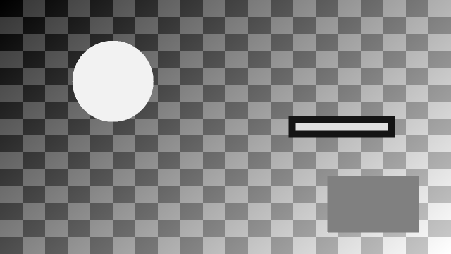
Summing the four input pixels increases the signal level and can improve the visibility of features in low-light conditions. At the same time, reducing the image dimensions decreases the memory bandwidth and processing required by later stages in the image-processing pipeline.

Because the output is the sum of four pixel values, the output data type must be wide enough to represent a value up to four times the maximum input pixel value.

Pixel binning may be used in applications such as:

• Astronomy

• Scientific cameras

• Low-light surveillance

• Medical imaging

• High-speed camera systems

• 
  

It is also useful when the full resolution of the sensor is not required, or when a smaller image must be processed at a higher frame rate.

Linear Smoothing

Linear smoothing reduces pixel-to-pixel variations by replacing each pixel with the average of the pixels in a surrounding 3×3 window.

For a nine-pixel window:

Pₒᵤₜ = (1/9) Σᵢ₌₁⁹ Pᵢ

Averaging neighbouring pixels reduces random noise and produces a smoother image. The trade-off is that edges are also softened and some fine image detail may be lost.

Linear smoothing can therefore be useful as a pre-processing stage before operations such as thresholding, edge detection, object tracking, or feature extraction. Reducing noise before these stages can help prevent small variations in pixel intensity from producing false detections.

Neighbouring pixels are averaged, making edges slightly softer and reducing small intensity variations. Overall brightness remains nearly unchanged.

Typical applications include:

• Industrial inspection

• Surveillance

• Robotics

• Camera pre-processing

• Medical imaging

• 
  

Median Filtering

Median filtering also operates on a neighbourhood of pixels, but instead of averaging the values, it sorts them and selects the middle value.

For a 3×3 window, the nine pixel values are collected and ordered, and the median value becomes the output pixel.

This makes the median filter particularly effective at removing impulse noise, which often appears as isolated bright or dark pixels.

Isolated black and white noise pixels are removed while normal regions and edges remain almost unchanged. The difference is subtle because only the deliberately corrupted pixels are corrected.

Unlike an averaging filter, an extreme pixel value does not significantly influence the result because the output is selected from the ordered pixel values rather than calculated from their sum. As a result, median filtering generally preserves edges better than linear smoothing.

Median filtering can be used to remove salt-and-pepper noise caused by:

• Sensor errors

• Transmission faults

• Electrical interference

  
  

Typical applications include industrial inspection, medical imaging, document processing, surveillance, and dead-pixel-correction systems.

Binary Image Thresholding

Binary thresholding converts a greyscale image into an image containing only two possible output values, typically black and white.

Each input pixel is compared with a selected threshold, in this example, the threshold is 128:

Pₒᵤₜ = 255 if Pᵢₙ ≥ 128

Pₒᵤₜ = 0 if Pᵢₙ < 128

Pixels with an intensity of 128 or greater become white, while pixels below 128 become black.

Pixels below 128 become black and pixels at or above 128 become white. Apparent grey regions are densely alternating black and white pixels being averaged by the viewer at reduced magnification.

The threshold therefore separates brighter regions of the image from darker regions.

Binary images are considerably simpler to analyse than full greyscale images.

Thresholding can therefore be used to isolate objects from their background or to generate a mask for later image-processing operations.

Typical applications include:

• Industrial inspection and defect detection

• Object-presence detection

• Barcode and text localisation

• Document scanning

• Cell or particle counting

• Image segmentation

• Creating masks for morphological processing

• Separating bright objects from a dark background

  
  

The choice of threshold is important. A low threshold classifies more pixels as white, while a higher threshold selects only the brightest pixels.

The most appropriate threshold depends on factors such as the sensor, lighting conditions, and the objects being detected. More advanced systems can calculate the threshold automatically or use different threshold values across different regions of the image.

Sobel Edge Detection

The Sobel algorithm detects boundaries by identifying rapid changes in image intensity.

It uses two 3×3 filters to measure intensity changes in the horizontal and vertical directions. These produce two gradients, conventionally referred to as (G_x) and (G_y).

The horizontal and vertical gradients are then combined to estimate the strength of an edge. Pixels whose edge strength exceeds a selected threshold can then be marked as edge pixels.

Sobel processing reduces an image to important structural information such as object outlines and boundaries. This information can then be processed more efficiently by later stages of a vision system.

Flat image regions become black, while strong brightness transitions become white outlines. This highlights object boundaries and checkerboard edges.

Typical applications include:

• Product inspection

• Object measurement

• Robot navigation

• Lane detection

• Alignment

• Barcode localisation

• Shape recognition

• 
  

For example, an industrial inspection system could use edge information to determine whether a manufactured component has the expected outline or dimensions.

Dark-Frame Subtraction

Image sensors can produce non-zero pixel values even when no light is reaching the sensor.

A dark frame is captured while the sensor receives no light and records unwanted background values caused by effects such as:

• Electronic offsets

• Leakage current

• Thermal effects

• Fixed-pattern sensor noise

• 
  

The stored dark-frame value is then subtracted from the corresponding pixel in each captured image:

Pcorrected = max(Pimage − Pdark, 0)

Any negative result is clamped to zero.

The stored sensor offset is removed, making the entire image slightly darker and correcting artificial bright regions. Object shapes remain unchanged.

Removing the unwanted background signal produces more accurate black levels and can make weak image signals easier to distinguish from sensor noise.

Dark-frame subtraction is particularly useful in applications that need to detect very low signal levels, including:

• Astronomy

• Fluorescence microscopy

• Scientific imaging

• Thermal imaging

• X-ray systems

• Long-exposure photography

• 
  

Dead-Pixel Correction

Image sensors may contain defective pixels that remain permanently bright, permanently dark, or fixed at an incorrect value.

A defect map can be used to identify the location of each known defective pixel.

Pixels that are operating normally pass through the processing chain unchanged. When the defect map indicates that a pixel is defective, its value is replaced using information from the surrounding pixels.

In this example, the defective pixel is replaced with the median value from its surrounding 3×3 neighbourhood.

 Isolated defective black or white pixels are replaced using neighbouring pixel values. Almost all other pixels remain unchanged.

The surrounding pixels provide a reasonable estimate of the missing value, while using the median helps prevent another unusually high or low pixel from being selected as the replacement.

Dead-pixel correction can be useful in almost any camera system, particularly:

• Industrial cameras

• Scientific instruments

• Astronomy cameras

• Medical imaging systems

• High-resolution image sensors

• 
  

Correcting these defects prevents persistent bright or dark dots from appearing in displayed images and helps prevent defective pixels from affecting image measurements.

Flat-Field Correction

Image sensors and optical systems do not always produce uniform brightness across the entire image.

Several effects can cause some areas to appear brighter or darker than others, including:

• Lens shading

• Differences in pixel sensitivity

• Dust

• Uneven illumination

  
  

Flat-field correction compensates for these variations by applying a position-dependent gain to each pixel:

Pcorrected(x,y) = Pinput(x,y) × G(x,y)

The gain map is normally calculated using an image of a uniformly illuminated surface.

Regions that appear darker receive a larger gain, while brighter regions receive a smaller gain. Fixed-point gain values can be used to implement the correction efficiently within the FPGA using multiplication and shift operations.

Darker edges and corners are brightened more than the image centre. This reduces lens shading and produces more uniform illumination.

Flat-field correction is commonly used in:

• Microscopy

• Astronomy

• Medical imaging

• Scientific instruments

• Document scanning

• Industrial inspection

It is particularly important in systems where pixel brightness is used as part of a measurement. Without correction, variations caused by the sensor or illumination could incorrectly be interpreted as real features within the scene.

Conclusion

The algorithms we have looked at demonstrate several different roles that image processing can perform within an FPGA-based imaging system.

Pixel binning can reduce image dimensions and increase signal levels. Linear and median filtering can reduce unwanted noise. Thresholding and Sobel edge detection can extract useful information for later analysis, while dark-frame subtraction, dead-pixel correction, and flat-field correction can compensate for imperfections in the sensor and imaging system.

Individually, these operations are relatively straightforward, but they can also be combined to create much more capable image-processing pipelines.

Using Simulink HDL Coder allows us to concentrate on developing and evaluating the processing algorithms before considering the generated RTL implementation. You can find the RTL and the Simulink models here.

FPGA Conference

FPGA Horizons London- October 6th and 7th 2026 - get Tickets here.

FPGA Journal

Read about cutting edge FPGA developments, in the FPGA Horizons Journal or contribute an article.

Workshops and Webinars:

If you enjoyed the blog why not take a look at the free webinars, workshops and training courses we have created over the years. Highlights include:

• Upcoming Webinars Timing, RTL Creation, FPGA Math and Mixed Signal

• Professional PYNQ Learn how to use PYNQ in your developments

• Introduction to Vivado learn how to use AMD Vivado

• Ultra96, MiniZed & ZU1 three day course looking at HW, SW and PetaLinux

• Arty Z7-20 Class looking at HW, SW and PetaLinux

• Mastering MicroBlaze  learn how to create MicroBlaze solutions

• HLS Hero Workshop  learn how to create High Level Synthesis based solutions

• Perfecting Petalinux  learn how to create and work with PetaLinux OS

Boards

Get an Adiuvo development board:

• Adiuvo Embedded System Development board - Embedded System Development Board

• Adiuvo Embedded System Tile - Low Risk way to add a FPGA to your design.

• SpaceWire CODEC - SpaceWire CODEC, digital download, AXIS Interfaces

• SpaceWire RMAP Initiator - SpaceWire RMAP Initiator,  digital download, AXIS & AXI4 Interfaces

• SpaceWire RMAP Target - SpaceWire Target, digital download, AXI4 and AXIS Interfaces

• Other Adiuvo Boards & Projects.

Embedded System Book   

Do you want to know more about designing embedded systems from scratch? Check out our book on creating embedded systems. This book will walk you through all the stages of requirements, architecture, component selection, schematics, layout, and FPGA / software design. We designed and manufactured the board at the heart of the book! The schematics and layout are available in Altium here.  Learn more about the board (see previous blogs on Bring up, DDR validation, USB, Sensors) and view the schematics here.

All words in this blog were written by a human.